Repeated positive-expectation gambles can have very negative actual outcomes
You shouldn’t ‘expect’ an expected value.
In this post we will explore how playing positive expected value games is not always a good idea, even if you can play them repeatedly. This runs counter to common beliefs regarding expected values. We lean on the excellent example from Ole Peters' article in Nature.
Consider a simple positive expectation game
Say you have a current wealth of
The expected value (EV) of this gamble is
- Do you take this gamble?
- What if you were offered the opportunity to play this game
- How much would you pay to play this game
I think the most common answer to the first two questions would be yes, at least for risk-neutral types. This is a risky gamble, but surely, we should expect to come out ahead given enough repetitions, it is a +EV gamble after all. After a quick calculation involving the compounding of the expected returns, I believe many people would pay a fortune to be offered the opportunity to play this game repeatedly.
With an initial bankroll of
This gamble is actually a terrible idea
Let’s see what actually happens when individuals take this gamble repeatedly.
 Figure 1. The blue line gives the expected wealth for the number of played rounds, while the thin red lines show the wealth trajectories for 100 players as they play 500 rounds. The solid red line is the typical wealth trajectory. Note the logarithmic scale.
In the plot above, the thin red lines show the wealth trajectories for 100 individuals who have chosen to play the game for 500 rounds, all starting with $1. The thick blue line represents the trajectory of expected wealth. The solid red line represents typical wealth trajectory, with its slope being the actual growth rate of this repeated gamble.
What’s going on here? Everyone is losing wealth, even though each gamble is +EV and the expected wealth path has a positive slope and grows rapidly.
This happens because the system is not ergodic
A naïve player of this game would expect to become fabulously wealthy in time based on his computation of the expected value, but we can see that anyone that repeatedly plays this game should actually expect to go broke.
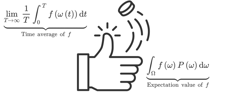
To understand why this is the case, we need to understand the concept of ergodicity. Very loosely speaking, an ergodic observable is one where the mean value for a group at any point in time is the same as the mean value for an individual over all times. Estimating the proportion of heads obtained by 1,000 people flipping a coin is equivalent to a single person flipping a coin 1,000 times, so the proportion is an ergodic observable.
An example of a non-ergodic observable would be the number of deaths obtained when playing Russian roulette. Asking 1,000 individuals to play a single round has a very different dynamic to asking one person to play 1,000 rounds in a row with the same gun. In this setting, the ensemble average is not the same as the time average.
The ordinary expected value we have computed for the gamble is an ensemble average. Due to the multiplicative dynamics of the gamble, path dependence plays an important role and wealth or even change in wealth are not ergodic observables. Therefore, the ensemble average (or space average) and the time average are not the same, and so it is not appropriate for an individual to apply the ensemble based expected value of wealth growth for decision making.
To be clear, the expected value of wealth is not wrong per se, with an infinite ensemble of players, the average wealth will indeed grow in time. But this is meaningless to an individual who does not benefit from the lucky members of the infinite ensemble who grow and stay wealthy.
How do we evaluate this gamble properly?
To understand if this gamble is a good idea or not, we need to identify an ergodic observable whose expectation value reflects the systems behaviour over time and not just over an ensemble. Under multiplicative dynamics, Peters (2015, eq. 5) shows that the rate of change in the logarithm of wealth is an ergodic observable
The fact that this quantity is ergodic means that when we compute the (ensemble) expected value, it will also reflect the behaviour of the observable in time and not just the mean value over infinite gamblers. Plugging our gamble in to this formula we obtain
Raising
Using the Kelly criterion
Assuming one has the prospect of being able to make many bets in time, the Kelly criterion can be used to estimate what proportion of wealth should be staked on any one gamble to maximise your long-term wealth. For simple gambles, the Kelly fraction, or the proportion of your current wealth that should be bet can be calculated as

We do not need expected utility theory
Expected utility theory is one way to approach decision making with probabilistic outcomes. However, utility theory ultimately leans on humans differing psychological responses to positive and negative outcomes as a framework
for decision making. One could absolutely chose (or craft) a utility function that produces equivalent results to maximising the geometric growth rate of wealth (changes in
I believe it is important to note that we do not have to invoke expected utility theory, risk-aversion, unknowable utility/loss functions, etc, to prevent us from losing money over time on this gamble, it suffices to just properly understand the dynamics.
Update on 2021-07-6: I believe this tweet from Ole Peters highlights this point well:
Wondering how deep this goes.
— Ole Peters (@ole_b_peters) July 5, 2021
What do you think viral evolution optimizes for, roughly?
a) time-average growth rate of # viral copies
b) one-shot multiverse-average (=expected value) of psychologically determined viral preferences expressed as a non-linear utility function
Evolution is clearly not maximising the utility function of successful viruses (they cannot express preferences after all). Under the multiplicative dynamics of virus replication, the force of evolution that optimises time-average growth rates ensures a virus’s success.
Lessons
The ordinary expected value we have computed for the gamble is an ensemble average, so the blue ‘expected growth’ line in figure 1 gives the average wealth over an infinite number of players, not what an individual player should expect. In this multiplicative, non-ergodic setting, the ‘expected’ in expected value is a complete misnomer.
It is thus not always wise to make repeated +EV decisions if the system is not ergodic or if there is a risk of ruin. However, this consideration does not seem to be widely understood or widely known:
If a game is ‘favorable’ from the point of view of the expectation value and you have the choice of repeating it many times, then it is wise to do so.
– H. Chernoff and L. E. Moses. Elementary Decision Theory.
Clearly, this statement is false.
Things to take away
- Understand if your system is ergodic. Is the time average of the observable equal to the ensemble average? (It probably isn’t).
- Don’t blindly optimise for expected value or ensemble averages, you might end up with terrible outcomes.
- You do not benefit from the positive outcomes observed by the other versions of you in ‘parallel universes’.
More
If you are interested in the ideas discussed in this post, gambles, expected values, ergodicity, utility theory and decision theory, check out these excellent papers:
and the blog:
Also check out
- The Logic of Risk Taking, a blog post by Nassim Nicholas Taleb (thoroughly recommended)
- Ergodicity-breaking reveals time optimal decision making inhumans
- Kelly Criterion (Wikipedia)
- Fortunes Formula: The Untold Story of the Scientific Betting System that Beat the Casinos and Wall Street (Book).